The release of Piter Pasma's Universal Rayhatcher has generated extensive interest in using signed distance functions (SDFs) for geometric modeling, and so I wanted to provide a deep dive into one output I created, explaining the entire formula step-by-step. The output I'm explaining here is Universal Rayhatcher #178, "A Truchet a day keeps the collector at bay".
To follow along, I suggest you try all the formulas I present here in the rayhatching development environment provided by Piter Pasma. Set the minter address to my Tezos address (tz1XTr7d3FZ19KndZ1HX3iav8fqKeZwGx8bZ) to get exactly the same views I'm getting. For simplicity, I've provided this setup for you at this link. You also have to set the correct title. I'm using "A Truchet a day keeps the collector at bay" (without quotes). Pay attention to the capitalization, as it modifies the random seed. Also, if you haven't read the documentation for the rayhatching code, I suggest you read it before proceeding.
Iteration #178 uses the concept of Truchet tiling. If this is the first time you're hearing this term, I encourage you to check out the Wikipedia article on the topic. In brief, Truchet tiling uses a set of square tiles that can be randomly combined to generate interesting patterns. Often, the tiles are designed such that any line that exits on one edge of any tile meets a line that enters on the opposing edge of any other tile. With this design, Truchet tiling can generate infinite, non-repeating patterns that look continuous and organic. There are many Truchet-based collections that have been released on fx(hash). Just go to "explore generators" and search for "Truchet" to find them.
Ok, so how do we generate a Truchet pattern in the rayhatching framework? Let's proceed step-by-step. The trick to developing complex SDFs is to progress in small steps and build up more complex scenes by combining individual elements that each are simple enough to understand.
The first step is always to just draw something, so we can see where the camera points to and where the light source is. I like to start with a sphere. The SDF for a sphere located at the origin is L(x,y,z)-r, where L stands for "length" and r is the sphere radius:
r=3;
L(x,y,z)-r
Note that I have set the background option to "none". Therefore we only see the sphere but no shadow.
Next, let's figure out tiling. We tile with the modulo operator (mod). Modulo is the remainder of a division. For example, 7 modulo 5 is 2. By applying modulo to one or more of our spatial coordinates x, y, and z, we subdivide space into cells that all have the same size. Here, I introduce a variable C that defines the size of the cells, and then transform x into x=mod(x,C)/C-.5. By dividing by C and then subtracting .5, I end up with x values within each cell that run from -0.5 to 0.5. Thus, after transformation, each cell is exactly 1 unit wide, and the center of each cell lies at x = 0. Because I have divided x by C, I need to similarly divide y and z by C, so that space overall is scaled in the same way. I also need to reduce the sphere radius so it still fits into a cell. Thus, this is my code to repeat the sphere infinitely many times along the x axis:
C=3,r=0.5;
x=mod(x,C)/C-.5,y=y/C,z=z/C,
L(x,y,z)-r
Note that the actual SDF, L(x,y,z)-r, has not changed from the previous step. Even though we see infinitely many spheres in the output, we only have a single sphere in the SDF. Instead of copying the sphere, we use the modulo operator to fold space into a single cell. This is a common theme when working with SDFs. We usually transform the spatial coordinates in all sorts of ways and then use very simple SDFs to create a shape in the transformed coordinates.
Next, let's tile space in two dimensions. This is a minor modification to the previous formula. We just need to apply modulo to both x and z. I could write out x=mod(x,C)/C-.5, z=mod(z,C)/C-.5, but instead I use the macro notation @xz{$=mod($,C)/C-.5,} which duplicates the formula twice and first replaces $ with x and then with z. You can see that that's the same as typing modulo separately for x and z.
C=3,r=0.5;
@xz{$=mod($,C)/C-.5,}
y=y/C,
L(x,y,z)-r
Now let's replace the sphere with rods. The SDF of a rod of radius r along the z axis is L(x,y)-r, and similarly L(z,y)-r for a rod along the x axis. If we want both, we can union them using the U() operator:
C=3,r=0.05;
@xz{$=mod($,C)/C-.5,}
y=y/C,
U(L(x,y)-r,L(z,y)-r)
This is all nice and good, but it's rather boring. We have subdivided space into many cells but each cell contains the exact same thing. In Truchet tiling, we need a different, randomly chosen tile in each cell. So how do we do this?
First, we need to know which cell we're in. Remember that I said modulo is the remainder of the division x/C. There is also the other component, the integer representing the number of times C fits into x, and we can calculate it with floor(x/C). For example, floor(7/5) = 1, floor(16/5) = 3, etc. These integers uniquely identify each cell. Since we're tiling in two dimensions, we need to perform this calculation for both x and z, and I'm calling the resulting indices ix and iz. I'm again calculating them using the macro trick, so that the macro line becomes @xz{i$=floor($/C),$=mod($,C)/C-.5,}.
Now that we know which cell we're in, what do we do with it? We generate a random number using the ri() function, and then draw either a sphere or rods depending on the value of the random number. I generate the random number with rn=ri(ix,iz,25)+.5. Here, the 25 is arbitrary and determines the final pattern. Change it to something else for a different random pattern. I add .5 to move the random number into the range of 0 to 1. (ri() produces random numbers between -.5 and .5.) The random choice is implemented via the JavaScript ternary operator condition ? exprIfTrue : exprIfFalse. Our condition is rn<.5, meaning half the time we get one output and half the time the other. Then, for exprIfTrue we draw a sphere, L(x,y,z)-5*r, and for exprIfFalse we draw rods, U(L(x,y)-r,L(z,y)-r). This is the final code:
C=3,r=0.05;
@xz{i$=floor($/C),$=mod($,C)/C-.5,}
y=y/C,
rn=ri(ix,iz,25)+.5,
rn<.5?L(x,y,z)-5*r:U(L(x,y)-r,L(z,y)-r)
Now I want to make one more modification to this code before moving on. I want to introduce functions a() and b() that represent a sphere or rods, respectively. The modified code looks like so:
C=3,r=0.05,
a=(x,y,z)=>L(x,y,z)-5*r,
b=(x,y,z)=>U(L(x,y)-r,L(z,y)-r);
@xz{i$=floor($/C),$=mod($,C)/C-.5,}
y=y/C,
rn=ri(ix,iz,25)+.5,
rn<.5?a(x,y,z):b(x,y,z)
The functions a() and b() are our two tiles, and the last line simply picks a random tile within each cell. This modification makes the code more readable, and it'll be even more important as we add more tiles.
In my final scene, I don't want spheres. Instead I want only straight and curved rods. To not have ugly breaks, where rods just end at the edge of a tile, I need tiles that provide smooth endpoints. Let's start with a tile that contains a smooth endpoint for each of the four rods that enter on each side of the tile. This requires the SDF for a line segment with finite length and smooth end. This SDF is a minor modification of the sphere SDF, via the clamp function cl(). We can think of clamp as stretching space. We write L(x-cl(x,0.3,0.5),y,z)-r, which is a sphere that in the x direction is stretched from 0.5 to 0.3. Remember, 0.5 is the edge of the tile. So the resulting rod starts at the right edge of the tile and extends 20% inwards, to the point 0.3. We encapsulate the rod statement into a function sg() (for segment), sg=(x,y,z)=>L(x-cl(x,0.3,0.5),y,z)-r.
The sg() function defines one rod, but how do we get a rod on either side of a cell? First, we can use the absolute operator B() to mirror the left side over. Thus, sg(B(x),y,z) creates a rod on both the left and the right side. Second, we can swap x and z, sg(B(z),y,x), to get rods on the other two edges.
This is the final result:
C=3,r=0.05,
sg=(x,y,z)=>L(x-cl(x,0.3,0.5),y,z)-r,
a=(x,y,z)=>U(sg(B(x),y,z),sg(B(z),y,x));
@xz{i$=floor($/C),$=mod($,C)/C-.5,}
y=y/C,
a(x,y,z)
Now let's add some tiles where rods go all the way through, and let's reintroduce the random tile choice:
C=3,r=0.05,
sg=(x,y,z)=>L(x-cl(x,0.3,0.5),y,z)-r,
a=(x,y,z)=>U(sg(B(x),y,z),sg(B(z),y,x)),
b=(x,y,z)=>U(sg(B(x),y,z),L(x,y)-r),
c=(x,y,z)=>b(z,y,x);
@xz{i$=floor($/C),$=mod($,C)/C-.5,}
y=y/C,
rn=ri(ix,iz,25)+.5,
rn<.5?b(x,y,z):c(x,y,z)
This is starting to look nice, but we need more tile variety. Let's add some tiles with curved paths. First, we can place a donut in the center of tile a(), to get four rods that connect into a circle. We do this via the donut operator unioned to the rest of the tile, like so: U(a(x,y,z),don(x,z,y,.3,r)). Next, let's make quarter donuts to connect rods that enter through two adjacent edges. This sounds like a difficult undertaking at first, but because we're tiling space we don't have to worry about any geometry that extends past the edges of a tile. Thus, we can make quarter donuts by simply placing complete donuts onto tile edges, like so: don(x-.5,z-.5,y,.5,r).
Thus, we arrive at curved paths and loops:
C=3,r=0.05,
sg=(x,y,z)=>L(x-cl(x,0.3,0.5),y,z)-r,
a=(x,y,z)=>U(sg(B(x),y,z),sg(B(z),y,x)),
b=(x,y,z)=>U(sg(B(x),y,z),L(x,y)-r),
c=(x,y,z)=>b(z,y,x),
d=(x,y,z)=>U(a(x,y,z),don(x,z,y,.3,r)),
e=(x,y,z)=>U(don(x-.5,z-.5,y,.5,r),don(x+.5,z+.5,y,.5,r));
@xz{i$=floor($/C),$=mod($,C)/C-.5,}
y=y/C,
rn=ri(ix,iz,25)+.5,
rn<.5?d(x,y,z):e(x,y,z)
Ok, so now we have five different tiles but we're only choosing two of them. How do we choose more? We can repeatedly apply the ternary operator. For example, we first test whether the random number is <0.25, and then we test whether it is <0.5, and so on. This results in the following (using four of the five tiles):
C=3,r=0.05,
sg=(x,y,z)=>L(x-cl(x,0.3,0.5),y,z)-r,
a=(x,y,z)=>U(sg(B(x),y,z),sg(B(z),y,x)),
b=(x,y,z)=>U(sg(B(x),y,z),L(x,y)-r),
c=(x,y,z)=>b(z,y,x),
d=(x,y,z)=>U(a(x,y,z),don(x,z,y,.3,r)),
e=(x,y,z)=>U(don(x-.5,z-.5,y,.5,r),don(x+.5,z+.5,y,.5,r));
@xz{i$=floor($/C),$=mod($,C)/C-.5,}
y=y/C,
rn=ri(ix,iz,25)+.5,
rn<.25?a(x,y,z):rn<.5?b(x,y,z):rn<.75?c(x,y,z):d(x,y,z)
The more tiles we have, the longer the last line. At some point it becomes unwieldy, so we may want to simplify with a macro. We write the comparison as rn<.25*i, where i = 1, 2, 3, 4. Here we use a little trick that you may know if you have ever programmed in C or C++: We write rn<.25*i++. This uses the current value of i in the comparison and then immediately increments i by one, so the next time we execute the same comparison i will be larger. The macro version of the code looks like this (output unchanged):
C=3,r=0.05,
sg=(x,y,z)=>L(x-cl(x,0.3,0.5),y,z)-r,
a=(x,y,z)=>U(sg(B(x),y,z),sg(B(z),y,x)),
b=(x,y,z)=>U(sg(B(x),y,z),L(x,y)-r),
c=(x,y,z)=>b(z,y,x),
d=(x,y,z)=>U(a(x,y,z),don(x,z,y,.3,r)),
e=(x,y,z)=>U(don(x-.5,z-.5,y,.5,r),don(x+.5,z+.5,y,.5,r));
@xz{i$=floor($/C),$=mod($,C)/C-.5,}
y=y/C,
rn=ri(ix,iz,25)+.5,
i=1,
@abc{rn<.25*i++?$(x,y,z):}d(x,y,z)
We can now just create more tiles and just use an ever longer macro call, such as @abcdefg{...}. However, when I wrote the original token I got a stack overflow error that I now can no longer reproduce. I'll quickly explain how I worked around this but I won't use the workaround for the remainder of this article.
What I did was write two separate conditions, first testing whether the random number is larger or smaller than 0.5, and then using the same macro trick separately within each 0.5-wide interval. The code looks as follows. Note that I've also added one more tile, f(), which places donuts on the opposite corners of e(). Also, note that by using rn<0.2*i I'm using uneven bin sizes for the different tile options. This is fine, it just generates a different output than if I were using even bins.
C=3,r=0.05,
sg=(x,y,z)=>L(x-cl(x,0.3,0.5),y,z)-r,
a=(x,y,z)=>U(sg(B(x),y,z),sg(B(z),y,x)),
b=(x,y,z)=>U(sg(B(x),y,z),L(x,y)-r),
c=(x,y,z)=>b(z,y,x),
d=(x,y,z)=>U(a(x,y,z),don(x,z,y,.3,r)),
e=(x,y,z)=>U(don(x-.5,z-.5,y,.5,r),don(x+.5,z+.5,y,.5,r)),
f=(x,y,z)=>U(don(x+.5,z-.5,y,.5,r),don(x-.5,z+.5,y,.5,r));
@xz{i$=floor($/C),$=mod($,C)/C-.5,}
y=y/C,
rn=ri(ix,iz,25)+.5,
i=1,
rn<.5?(@ab{rn<.2*i++?$(x,y,z):}c(x,y,z)):(@de{rn<.5+.2*i++?$(x,y,z):}f(x,y,z))
Ok, now let's switch gears for a moment and talk about the floor. So far we have just generated the Truchet pattern, but it's nice to have it above a floor so we can see a shadow. In general, the SDF for a floor is simply y-h, where h is the y value at which the floor is located. We can make the floor a bit more interesting though if we add a bit of noise, using the nz() function. This looks as follows:
C=3,r=0.05,yt=1.8,yf=-5,
@xz{i$=floor($/C),$=mod($,C)/C-.5,}
y=y/C-yt,
y+yt-yf+.6*nz(x+ix,0,z+iz,.2,4)
You may be confused why I'm keeping all the x, y, and z transformations before the formula for the floor. That's because ultimately I want to combine this code with the Truchet tiling code. Also, I have introduced constants yt and yf. yt is the y value of the Truchet pattern, and yf is the y value of the floor. Finally, you may wonder about x+ix and z+iz. This is because nz() needs a global x and z, not tiled, but x and z are tiled at this point in the code. So we have to untile. Remember that both x and ix were derived from the division x/C, and adding x and ix recovers the original value (scaled by the constant C). Alternatively we could have made a copy of the original x value, but writing x+ix requires fewer characters. Thus, in the spirit of Piter Pasma's code minimization efforts, that's what we do here.
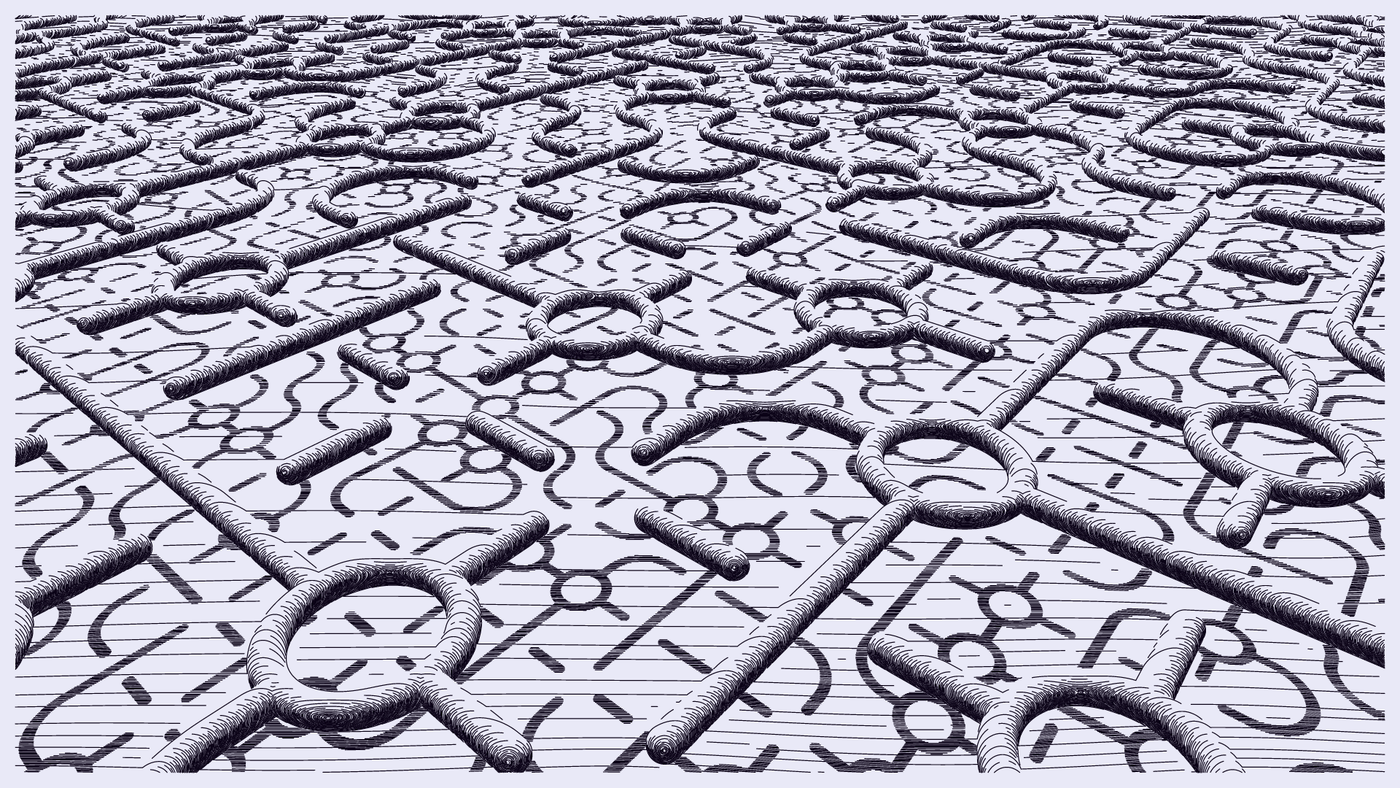
Now we can put everything together and end up with a Truchet tiling above a slightly undulating floor. In this final version, I'm using rn<.1667*i to obtain even probability bins for all tiles.
C=3,r=.05,yt=1.8,yf=-5,
sg=(x,y,z)=>L(x-cl(x,0.3,0.5),y,z)-r,
a=(x,y,z)=>U(sg(B(x),y,z),sg(B(z),y,x)),
b=(x,y,z)=>U(sg(B(x),y,z),L(x,y)-r),
c=(x,y,z)=>b(z,y,x),
d=(x,y,z)=>U(a(x,y,z),don(x,z,y,.3,r)),
e=(x,y,z)=>U(don(x-.5,z-.5,y,.5,r),don(x+.5,z+.5,y,.5,r)),
f=(x,y,z)=>U(don(x+.5,z-.5,y,.5,r),don(x-.5,z+.5,y,.5,r));
@xz{i$=floor($/C),$=mod($,C)/C-.5,}
y=y/C-yt,rn=ri(ix,iz,25)+.5,i=1,
tr=@abcde{rn<.1667*i++?$(x,y,z):}f(x,y,z),
U(tr,y+yt-yf+.6*nz(x+ix,0,z+iz,.2,4))
And there you have it. The final formula may seem completely incomprehensible, but every step along the way was hopefully manageable, and now that you look at the final result you can identify the individual pieces and see what they do. If you're trying to develop your own SDFs, I encourage you to take similarly tiny steps and make one small increment at a time. SDFs are not things that you just manipulate randomly to see what happens. To get specific results, you need to understand every concrete change that you make.
If you enjoyed this article and would like to get better at writing SDFs, where can you learn more? SDFs are commonly used in the shader world, and there are many resources to learn about them. I have previously written a blog post that explains these resources, so I'll just point you there. I would specifically encourage you to watch live-coding videos of people doing SDF-based modeling, as you can see in real time how they build a complex scene from the basic building blocks.
I hope you found this useful, and I'm looking forward to seeing your own SDF-based designs. All code examples in this article are licensed CC0, so you can use them in your own work as you see fit. Just remember: You shouldn't just take my SDF and mint your own token with it, even if the license allows you to do this. Instead, take the concepts I've described here and make them your own. Create your own art from the building blocks you've been given.