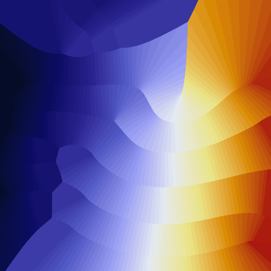
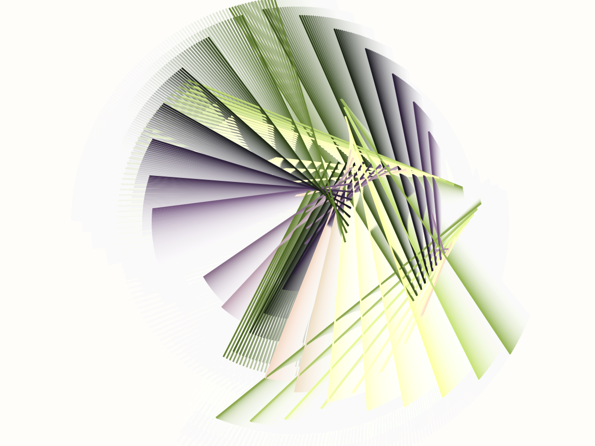
The Artifact continues my exploration of using t-distributed stochastic neighbor embedding (t-SNE) to generate art. The specific visualization chosen in The Artifact makes many of the iterations look like they are depictions of physical objects made out of a combination of a metal and some colorful, matte material. While iterations often may look like they are illuminated by light, the generative algorithm does not use any lighting model or calculations. The effect comes solely from deliberate use of color gradients within each piece.
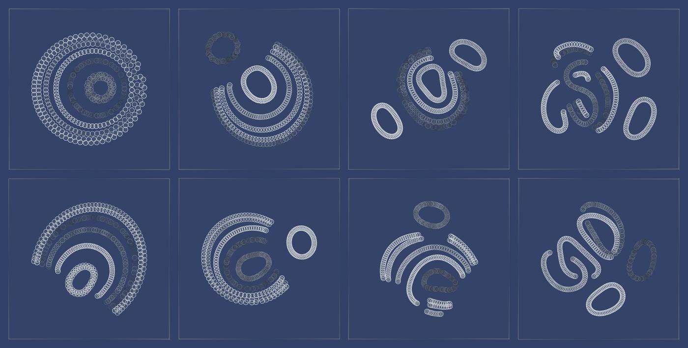
The algorithm used in The Artifact is deceptively simple. I start with an array of dots, for example arranged in wavy lines. I consider each line to be a "group," and every group contains the same number of dots. This input data is then transformed into a new arrangement of dots via t-SNE. This output arrangement is responsible for the geometric shapes of a given piece.
Now, I take this output arrangement of points and derive two sets of polygons from it. For the first polygon layer, I identify consecutive sets of points that are separated in space from other such sets of points and use them as polygon boundaries. For the second layer, I take all points in the output data and treat them as one large polygon boundary. In both cases, I render all polygons with the "evenodd" fill rule, so that self-intersections create interesting internal gaps in the polygons. Actually, the second layer is generated via one of two alternative options, which are listed as either "connected" or "fractured" in the features of the piece. In the "connected" option all points form one single polygon boundary. By contrast, in the "fractured" option all points belonging to one group form a separate polygon boundary.
At final rendering, the algorithm draws the two polygon layers above a background layer. The background layer is just a subtle color gradient, created by placing a cloud of points of one color on top of a solid rectangle drawn in a different color. In the first polygon layer, all polygons are drawn with solid fill, with colors varying depending on the group to which a polygon belongs. Importantly, all fill colors have some amount of transparency, so that the background shines through and creates some additional texture. By contrast, in the second polygon layer the polygons are drawn by randomly throwing dots onto the canvas and retaining only those dots that are inside the polygon boundary. The dot locations are generated via normal distributions. A normal distribution generates a density gradient such that more points are placed towards the center of the distribution and the further away from the center we go the fewer points remain. To render the second polygon layer, I am using three separate normal distributions with different center locations, and the points belonging to each distribution can have a different color. This setup generates the foreground color gradient that is so prominent in most of the iterations.
As you go through the iterations, you may notice that they can look very varied. However, all outputs are generated by the exact same algorithm, described above. Variation comes from different types of input data, different settings for t-SNE (most importantly the perplexity parameter, which determines how organized or disorganized the output is, but also the random seed, as t-SNE is not a deterministic algorithm), and different color palettes. Some iterations also apply some noise to the input data for added variation. You may also notice that the algorithm can sometimes go a bit crazy and produce some truly weird output. I have spent countless hours to fine-tune parameter settings to curate output quality, but sometimes the only difference between a spectacular output and a not-so-exciting one is literally just the random seed given to t-SNE. t-SNE is a beast that can be somewhat tamed but never fully controlled. I think the best way to deal with this remaining luck of the draw is to be prepared to mint a few iterations. Edition sizing and price have been chosen with that in mind.
History and implementation details
The Artifact is the culmination of 14 months learning JavaScript and making browser-based art, and in many ways it is my first fx(hash) release where I have not felt overly limited by the medium. The core idea for The Artifact predates any of my browser-based work. I first developed the algorithm in late 2021, using R. In November 2021 I minted the collection Shards of Blue on objk.com which you will recognize as obviously related to outputs generated by The Artifact. Because it was written in R, I needed to generate outputs offline, curate, and release rendered images in PNG format.
When fx(hash) beta opened I first dismissed it as a publishing venue for myself because I had never written a line of JavaScript in my entire life, and also I was using fairly advanced statistical tools such as t-SNE as generative algorithms and there was no good (and fast!) way to do t-SNE in the browser. But eventually, in early December, I decided to just give it a try and see where I would go. I made my first commit to my private GitHub repo containing JavaScript experiments on December 9, 2021, a simple p5 sketch drawing a 3D scene with a plane and a sphere.
I spent the next two weeks feverishly implementing the t-SNE algorithm in JavaScript and generally reproducing in JavaScript an idea I had previously played around with in R, where I used the output of the t-SNE transformation as centers of Voronoi cells. This turned into Sneronoi, which I released on December 26, 2021.
While Sneronoi was fundamentally a fine release, it had several technical issues I wasn't happy with. Most importantly, the t-SNE algorithm was rather slow, which required me to do something between the time the user opened the token to the time t-SNE was fully converged and the artwork considered final. My solution was the initial Sneronoi animation, where you can see the t-SNE algorithm doing its thing. It works, but to me it creates the impression that Sneronoi is an animated piece when it is not meant to be one, and I don't like that. Also, Sneronoi uses D3 for rendering, which I found easier to use than p5.js, coming from the R world. But, D3 is a massive library, and I didn't exactly understand what it was doing under the hood, so I didn't find using it ideal.
I released two more tokens using the same t-SNE implementation that I felt was overly slow, and then I decided I needed something better. That's when I started looking into WebAssembly (WASM). I eventually discovered AssemblyScript, which is a JavaScript-like language that can be compiled into WASM, and I found that with relatively modest amounts of work I could turn my JavaScript t-SNE implementation into AssemblyScript and obtain a meaningful speed increase.
The first work I released using the WASM implementation was Eternal Connection. In Eternal Connection, t-SNE convergence was so fast that I didn't need an animation and could instead just show a little progress bar. I also got rid of my D3 dependency and instead was just generating SVG output directly from my JavaScript code. Finally, this token involved much more careful curation and fine-tuning of the t-SNE algorithm and the data fed into the algorithm. I probably generated and reviewed 50,000 test outputs before I released the collection.
Yet there were technical issues I still wasn't happy with. Most importantly, I tried to add a textured background and ran into limitations of what can be done with SVG. For very detailed backgrounds, rendering the SVG would get very slow or even crash my browser. So I ended up making some visual choices that were not so much driven by artistic intent but rather by technical limitations. While I like the SVG format and the idea of generating a resolution-independent output that can be downloaded and stored as a perfect-quality archival version of the artwork, I have to accept that finely detailed outputs simply aren't possible in this format and require a bitmap-based approach instead. In the browser, this generally means working with the HTML Canvas.
The Canvas is great once you actually understand it. A light-bulb moment for me was discovering that you can set the size of the Canvas in pixels separately from the size at which it is shown in the browser. This means you can render a single, high-resolution image and then have it adapt and rescale to the size of the current browser window. In fact, this approach is critical to getting decent results on any modern Mac with retina displays, where the actual screen has a much higher resolution than is logically presented to the browser. I got comfortable with these ideas and with talking directly to the Canvas in the animated piece The Passing of Time.
Finally, The Artifact introduces a couple of additional technical ideas that I had not used in any prior fx(hash) piece. First, I have implemented progressive rendering, where the final image is assembled in hundreds of small steps without freaking out the browser in the meantime. (Browsers don't like it when JavaScript functions take more than a few miliseconds to execute.) In my progressive rendering pipeline, I first assemble a list of all the elements I eventually want to draw, and then on every iteration I draw one element of that list and return control back to the browser. Second, I am rendering different layers into different canvases and then combining them to create the final image. This is not strictly necessary for the final output generated by The Artifact, but it allows me to render the background only after some of the foreground elements have already been drawn, and this creates a better impression to the viewer that something is actually happening during the rendering stage.
The Artifact is also the first of my tokens whose behavior can be modified via URL parameters. The possible parameter options are listed in the token description. I would specifically encourage you to try appending &r=2&d=2 to the URL to generate a very high-resolution render with very fine stippling. Alternatively, if you're in a rush, use &r=0.5&d=0.5 for a coarse, quick render.
I have released the entire code to The Artifact into the public domain, under CC0. You can explore it here: https://github.com/clauswilke/artifact